In past installments of this series, we've talked a lot about the sharpness of the training loss Hessian, that is, the curvature in the most-curved direction. For any given choice of parameters, there are as many directions you can move as there are parameters, which for a typical neural network means millions to billions. For any direction you choose, there is both a slope - the amount that the loss is increasing or decreasing in that direction - and a curvature - the amount that the slope is increasing or decreasing in that direction. The curvature is measured by the eigenvalues of the Hessian matrix of the training loss; each eigenvalue corresponds to the curvature in one direction. The sharpness is the maximum curvature out of all of those millions of directions. Today we're going to literally go in a different direction: we're going to talk about the directions with very little curvature, and why that happens. Specifically, this post is an explication of a recent paper by Kühn and Rosenow, who I think have nailed this down, and who were kind enough to also answer some followup questions by e-mail.
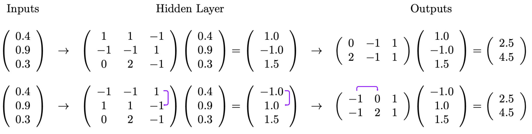
The core of Kühn and Rosenow's argument has to do with symmetry. We've known for a long time that there exists more than one way for a neural network to express a given function. For example, suppose we have a multilayer perceptron. If we swap two rows in one weight matrix and the corresponding columns in the next layer's weight matrix, along with the corresponding parts of the bias term, the effect is to swap two coordinates in the activations, without actually changing anything else. For example, suppose for some input, the first two coordinates of the activations in the original network are 1 and -1. After the swap, they'll be -1 and 1, but all the other activations - including the network outputs - will be the same. The network is expressing exactly the same function, but with different parameters. This is called a symmetry in the weight space. This sort of swap is the simplest kind, but far from the only one.
Kühn and Rosenow take this a step further, to approximate symmetries. Let's pretend for the moment that we have a neural network with no activation functions. For simplicity, we'll assume we have no bias terms, just weight matrices. At each layer, we take the output of the previous layer, multiply it by a matrix, and pass it on to the next layer. Suppose we left-multiply the weight matrix of one layer by some arbitrarily chosen matrix, and right-multiply the weight matrix of the next layer by its inverse. This has no effect at all on the outputs. The activations of that layer have been linearly transformed, but the transformation is immediately undone by the next layer, and everything afterwards proceeds as if it had never occurred. Any such matrix thus corresponds to a direction in parameter space where the slope and curvature are zero - moving in that direction has no effect at all on the loss. That means there's a corresponding zero eigenvalue of the Hessian matrix. Since we can do this for any invertible matrix and any hidden layer, this translates to a lot of zero eigenvalues - most of the eigenvalues, in fact.
But this only works in a network with no activation functions. If you have activation functions, the inverse matrix can't magically undo the effect of the matrix. Kühn and Rosenow's core insight is that while these directions don't translate to no change in the function, they still translate to very little change, meaning they have very little curvature. They show this through a clever trick where they interpolate between the network with no activation functions and the network with activation functions. For any activation function, we can define a smooth path between the function and doing nothing, allowing us to slowly shift from one to the other. Since the path is smooth, the change in the curvatures should be smooth too. With no activation functions, we know analytically how many zero curvature directions there are, and we can watch what happens as we shift from one to the other.
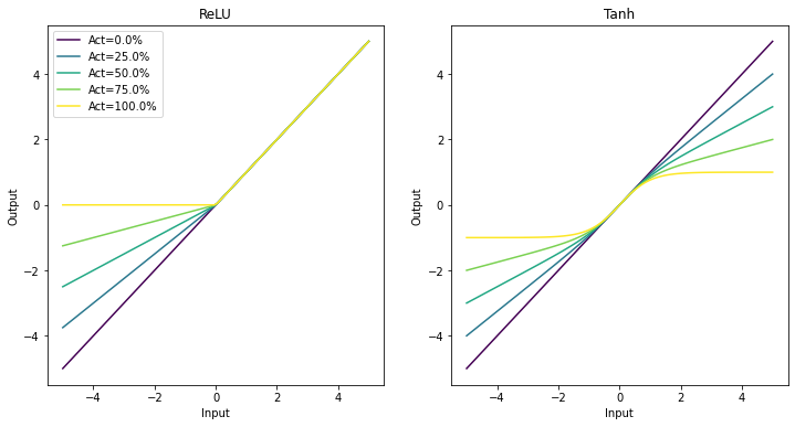
I figured I'd replicate what they did on a simpler example. I used the moons dataset, which is a standard synthetic toy dataset with two classes and two-dimensional inputs. I used a four-layer multilayer perceptron with either ReLU or tanh activations and a hidden dimension of 64. I chose a simple dataset and a small network so that I could materialize the Hessian matrix entirely instead of needing to use a Lanczos solver; the downside is that means my network needs to be very small indeed, and we don't see much change in the curvature during training because it takes so little time to memorize the data.
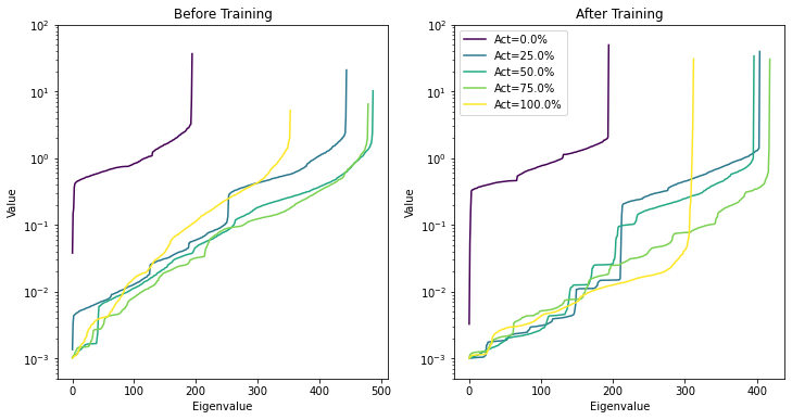
Below, I plot the eigenvalues before (left) and after (right) training. Each curve corresponds to a point along the interpolation between a no-activation network (purple) to the full activation network (yellow). I omit the negative eigenvalues so I can use a log scale. Due to floating point error, even zero eigenvalues end up being assigned some non-zero value; I (somewhat arbitrarily) picked 0.001 as the cutoff to declare an eigenvalue zero. First, here are the eigenvalues with ReLU activations:
And here are the eigenvalues with tanh activations:
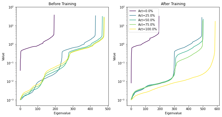
So when the activations are completely turned off, we have lots of zero eigenvalues. As we turn the activations back on, some of those zero eigenvalues stop being zero, but they remain relatively small. I find the left plots, from before training, especially interesting. Look at how each of the curves with activations turned on look like the curve with activations turned off, only with an extra set of non-zero eigenvalues below - and those added non-zero eigenvalues are roughly linear in the log plot, implying they follow a power law. This is a result that's been seen before (Tang et al. 2025), but in that case they only saw the power law emerge after training, not before. Right now, as far as I know, no one knows where that power law comes from.
One implication of this result that I think is that we need to add a new category to our understanding of the Hessian eigenvalues. Traditionally, we've seen the eigenvalues separate into a "top" and a "bulk". The top consists of a few large outliers, typically one for every dimension of the network output. The bulk is everything else, and there's usually a clear gap between the top and the bulk (Saarinen et al. 1993, Sagun et al. 2017, Sagun et al. 2018). These symmetric eigenvalues account for the majority of the bulk, not all of it, suggesting that we need to further separate the bulk into components, one corresponding to these symmetries and one not. This is not the first time something like this has been proposed - Papyan 2020 suggested calling the intermediate eigenvalues the "mini-bulk" - but this provides a pretty rigorous justification for why the bulk and the mini-bulk separate.
Overall, one of my favorite papers so far this year; I'm looking forward to seeing what else Kühn and Rosenow come up with.