The Gillespie Algorithm
Theory
A spatial stochastic system consists of a graph where each vertex of the graph has an associated state selected from a finite list of integers. Each vertex represents some piece of ecological real estate, and the state denotes its current occupants; traditionally 0 denotes an empty site, 1 denotes an individual of species 1, etc. The system evolves over time as a continuous-time Markov chain: for every pair of adjacent sites in states \(s_1, s_2\), the time until that pair transitions to states \(s_1', s_2'\) is an exponentially distributed random variable whose rate \(\rho(s_1, s_2\to s_1', s_2')\) is a function solely of \(s_1, s_2, s_1', s_2'\).
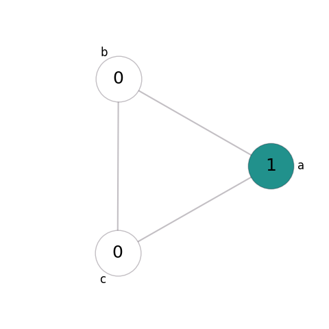
For example, suppose that our system consists only of empty sites (state 0) and a single species (state 1). We’ll give this system two possible transitions: reproduction and mobility. For simplicity, we’ll say that this is taking place on a fully-connected graph of 3 nodes, with initial state:
In reproduction, an individual of the species gives birth into an empty adjacent site - so a pair of adjacent sites in states 0 and 1 changes to both being in state 1:
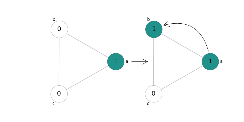
Let’s say this happens at rate 0.2. We write this in shorthand as \((0, 1)\to(1, 1)@0.2, (1, 0)\to(1, 1)@0.2\). In practice, we usually assume that our graphs are non-directed and all transitions are symmetric, and only write \((0, 1)\to(1, 1)@0.2\).
In mobility, two sites swap states. Since this has no effect if the sites are already in the same state, we only consider the case where sites with different states swap their contents:
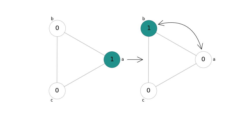
Let’s say this happens at rate 0.15. We write this in shorthand as \((0, 1)\to(1, 0)@0.15, (1, 0)\to(0, 1)@0.15\).
Before we continue, there’s a little bit of a subtlety here in how we define rates: is this the rate at which an event happens on an edge, or the rate at which it happens on an ordered pair? We know that the rate which \(a\) reproduces into \(b\) is 0.2. But is the rate at which \(a\) and \(b\) swap contents 0.15 - we have an edge, and the endpoints of that edge swap their contents, which is a single possible transition at rate 0.15? Or is it 0.3 - we have two ordered pairs, \((a, b)\) and \((b, a)\), and so we have two swapping transitions, both occurring at rate 0.15 with equal results? We use the latter interpretation, both because it simplifies the underlying code structure, and because it makes it more natural to allow directed graphs.
Now consider what happens. There are three edges, or six ordered pairs, in our graph: \((a, b), (b, a), (a, c), (c, a), (b, c), (c, b)\). Both ends of the \((b, c)\) edge are in state 0, so no transition there is possible under our rules. But we have six possible transitions:
Site \(a\) could give birth into site \(b: (1, 0)\to(1, 1)\).
Site \(a\) could give birth into site \(c: (1, 0)\to(1, 1)\).
Site \(a\) and \(b\) could swap: \((1, 0)\to(0, 1)\).
Site \(b\) and \(a\) could swap: \((0, 1)\to(1, 0)\).
Site \(a\) and \(c\) could swap: \((1, 0)\to(0, 1)\).
Site \(c\) and \(a\) could swap: \((0, 1)\to(1, 0)\).
So what happens? The time until any of these events happen is an exponentially distributed random variable with the specified rate. We could generate those random numbers and see which happens first, put that change into effect, then regenerate all our random variables and repeat. For example:
>>> import numpy as np
>>> np.random.exponential(0.2)  #  Event 1: a gives birth into b

0.0164659

>>> np.random.exponential(0.2)  #  Event 2: a gives birth into c

0.0620006

>>> np.random.exponential(0.15)  #  Event 3: a swaps with b

0.0403296

>>> np.random.exponential(0.15)  #  Event 4: b swaps with a

0.1017322

>>> np.random.exponential(0.15)  #  Event 5: a swaps with c

0.1908576

>>> np.random.exponential(0.15)  #  Event 6: c swaps with a

0.1052524
So the first event that happens is that \(a\) swaps with \(b\):

Now we have a whole new set of possible transitions. We could then recalculate all the possible transitions, look up their rates, and generate a whole new mess of random variables…
Practice
But that would take forever, and we want to publish some time this century. So instead we’re going to use the Gillespie algorithm.
The Gillespie algorithm is based on the observation that, given a collection of \(N\) events \(E_1, E_2, ..., E_n\), where the time to each event are exponentially distributed random variables with rates \(r_1, r_2, ..., r_n\), the time until some event \(E^*\) occurs is exponentially distributed with rate \(r_1 + r_2 + ... + r_n\), and which event occurs is a categorically distributed random variable with probabilities:
We start by calculating the maximum rate at which any ordered pair can go through any transition. So in our toy example, that is 0.35: the pair \((0, 1)\) can go through swapping (rate 0.15) or reproduction (rate 0.2). (Similarly the pair \((1, 0)\).) We pad our list of possible transitions with pseudotransitions from the pair to itself so that every possible ordered pair of states has the same total rate. So in our case, we add the following pseudotransitions:
\((0, 0)\to(0, 0)\) at rate 0.35.
\((1, 1)\to(1, 1)\) at rate 0.35.
So, under the Gillespie algorithm, the rate at which some transition or pseudotransition occurs is \(6 \cdot 0.35 = 2.1\). We could then roll an exponentially distributed random variable with that rate to determine the time until the next transition occurs, then select a random event by selecting a random ordered pair of vertices, and then selecting the transition proportional to the rate.
Let’s rewind to the original state of our graph:

We roll an exponentially distributed random variable with rate 2.1:
>>> import numpy as np
>>> np.random.exponential(2.1)

3.8921261
And then randomly select a random pair of events:
>>> import random
>>> random.choice(['a', 'b', 'c'])

'c'

>>> random.choice(['a', 'b'])

'a'
If we had selected b, then nothing would have happened since the only transitions for the pair \((0, 0)\) are pseudotransitions. But since we selected a, we have two possible transitions. The probability of the transition \((0, 1)\to(1, 1)\) is \(0.2 / 0.35 = 0.5714\), while the probability of the transition \((0, 1)\to(1, 0)\) is \(0.15 / 0.35 = 0.4286\). So we roll a uniform random variable:
>>> random.uniform(0, 1)

0.138
Getting reproduction:

In general, we don’t actually care about the elapsed time; we are primarily interested in the asymptotic state of the system. Therefore, we don’t bother actually generating the exponential random variable for the time: instead we just use the average value. Since a typical simulation will consist of millions of steps, this is a very good approximation.
The Diffusion Trick
There’s one further trick we can use, thanks to Reichenbach, Mobilia and Frey 2008. Most of the systems we’re interested in include diffusion - two individuals swapping places - as a frequent reaction. In fact, it will often be much more common than any other reaction. If the rate of diffusion is \(r_d\), and the maximum total rate for non-diffusion reactions is \(r_n\), then the number of diffusion events between non-diffusion events is a geometric random variable with \(p=r_d / (r_d + r_n)\). We can make the simulation more efficient by drawing from that geometric distribution, performing that many diffusion operations, and then performing a single non-diffusion operation.
However, there is one slight caveat: we use a set of pre-calculated thresholds to efficiently perform the geometric sampling. This is more efficient, but means there is a maximum number of possible diffusion events between non-diffusion events. The default maximum is very high (1024), and it should be very rare that the number of diffusions would exceed this, but it can potentially happen. If you’re concerned about this, you can do one of two things:
Pass the argument allow_diffusion_trick=False when calling the Geography.run method. This turns off the diffusion trick, at some cost in runtime.
Change the value MAX_DIFFUSIONS in the file graph_ops.h to a higher value, then reinstall the package.